Презентация на тему: Excel Tutorial 7

Excel Tutorial 7Using Advanced Functions, Conditional Formatting, and Filtering

Objectives Evaluate a single condition using the IF functionEvaluate multiple conditions using the AND functionCalculate different series of outcomes by nesting IF functionsTest whether one or more conditions are true with the OR functionReturn values from a table with the VLOOKUP function Check for duplicate values using conditional formatting

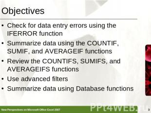
Objectives Check for data entry errors using the IFERROR functionSummarize data using the COUNTIF, SUMIF, and AVERAGEIF functionsReview the COUNTIFS, SUMIFS, and AVERAGEIFS functionsUse advanced filtersSummarize data using Database functions

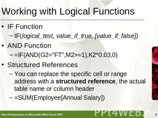
Working with Logical Functions IF FunctionIF(logical_test, value_if_true, [value_if_false])AND Function=IF(AND(G2="FT",M2>=1),K2*0.03,0)Structured ReferencesYou can replace the specific cell or range address with a structured reference, the actual table name or column header=SUM(Employee[Annual Salary])

Working with Logical Functions

Working with Logical Functions A nested IF function is when one IF function is placed inside another IF function to test an additional condition=IF([Pay Grade]=1,2500,IF([Pay Grade]=2,5000, IF([Pay Grade]=3, 7500,"Invalid pay grade")))

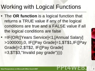
Working with Logical Functions The OR function is a logical function that returns a TRUE value if any of the logical conditions are true and a FALSE value if all the logical conditions are false=IF(OR([Years Service]<1,[Annual Salary]>100000),0, IF([Pay Grade]=1,$T$1,IF([Pay Grade]=2,$T$2, IF([Pay Grade]=3,$T$3,"Invalid pay grade"))))

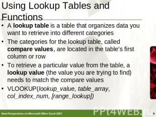
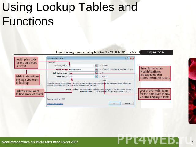
Using Lookup Tables and Functions A lookup table is a table that organizes data you want to retrieve into different categoriesThe categories for the lookup table, called compare values, are located in the table’s first column or rowTo retrieve a particular value from the table, a lookup value (the value you are trying to find) needs to match the compare valuesVLOOKUP(lookup_value, table_array, col_index_num, [range_lookup])

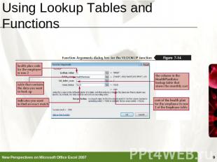
Using Lookup Tables and Functions

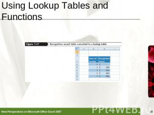
Using Lookup Tables and Functions

Highlighting Duplicate Records with a Custom Format Select the column you want to search for duplicatesIn the Styles group on the Home tab, click the Conditional Formatting button, point to Highlight Cells Rules, and then click Duplicate ValuesClick the values with arrow, then click Custom FormatIn the Format Cells dialog box, set the formatting you want to useClick the OK button in each dialog box

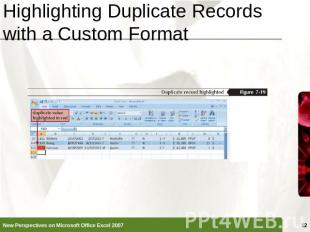
Highlighting Duplicate Records with a Custom Format

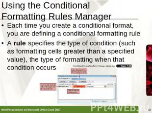
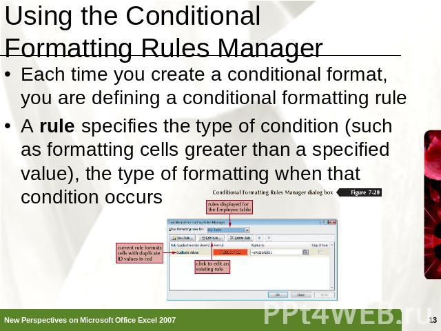
Using the Conditional Formatting Rules Manager Each time you create a conditional format, you are defining a conditional formatting ruleA rule specifies the type of condition (such as formatting cells greater than a specified value), the type of formatting when that condition occurs

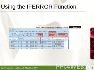
Using the IFERROR Function Error values such as #DIV/0!, #N/A, and #VALUE! indicate that some element in a formula or a cell referenced in a formula is preventing Excel from returning a calculated valueThe IFERROR function can determine if a cell contains an error value and display the message you choose rather than the default error value=IFERROR(VLOOKUP(L2,HealthPlanRates,2,False)*12,"Invalid code")

Using the IFERROR Function

Summarizing Data Conditionally You can calculate the number of cells in a range that match criteria you specify using the COUNTIF function, which is sometimes referred to as a conditional count=COUNTIF(range,criteria)You can add the values in a range that meet criteria you specify using the SUMIF function, which is also called a conditional sum=SUMIF(range,criteria[,sum_range])

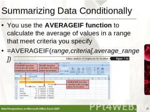
Summarizing Data Conditionally You use the AVERAGEIF function to calculate the average of values in a range that meet criteria you specify=AVERAGEIF(range,criteria[,average_range])

Summarizing Data Conditionally The COUNTIFS function counts the number of cells within a range that meet multiple criteriaCOUNTIFS(criteria_range1,criteria1[,criteria_range2,criteria2...])The SUMIFS function adds values in a range that meet multiple criteriaSUMIFS(sum_range,criteria_range1,criteria1[,criteria_range2, criteria2...])The AVERAGEIFS function calculates the average of values within a range of cells that meet multiple conditionsAVERAGEIFS(average_range,criteria_range1,criteria1[,criteria_range2, criteria2...])

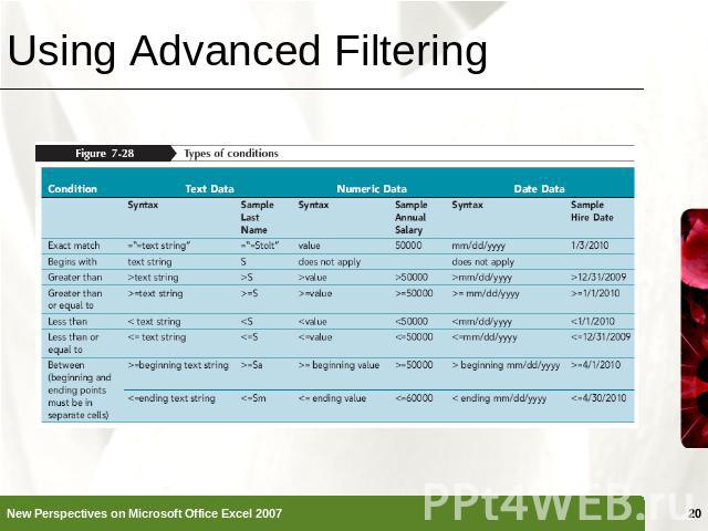
Using Advanced Filtering Advanced filtering, similar to filtering, displays a subset of the rows in a table or range of dataThe criteria range is an area in a worksheet, separate from the range of data or Excel table, used to specify the criteria for the data to be displayed after the filter is applied to the table

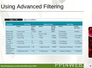
Using Advanced Filtering

Using Advanced Filtering Click the Data tab on the Ribbon, and then, in the Sort & Filter group, click the Advanced button

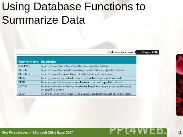
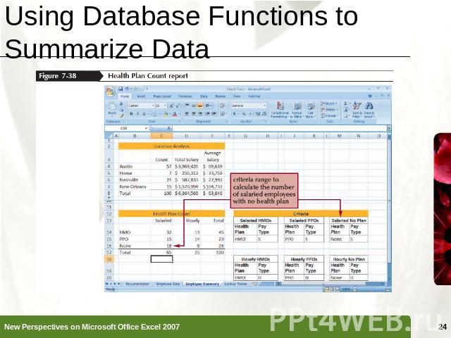
Using Database Functions to Summarize Data Functions that perform summary data analysis (SUM, AVERAGE, COUNT, and so on) on a table of values based on criteria that you set are called the Database functions, or DfunctionsDfunctionName(table range, column to summarize, criteria range)

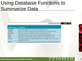
Using Database Functions to Summarize Data

Using Database Functions to Summarize Data